图像算法--轻量级CNN，MobileNet V1神经网络

MobileNet卷积神经网络

卷积神经网络存在什么问题？

首先大家要了解原始的卷积神经网络在进行多通道卷积的时候到底是怎么执行的。

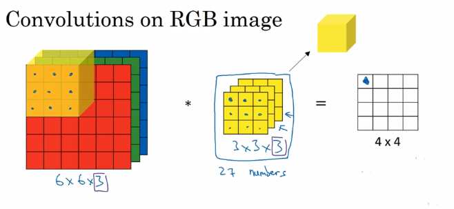
我们有个三通道的RGB图片，这个时候我们使用一个 $3\times 3\times 3$ 的卷积核来卷积这个图片，很明显最后一个，我们每次卷积都是27个参数一起训练，然后这个卷积核扫描原始的图片一次以后就生成了 $4 \times 4$ 的一个feather map，所以我们在实现卷积神经的时候都是使用更多个卷积核来形成一个 $4\times 4\times N$ 的一系列feather map。

问题

原始的卷积神经网络对应图像区域中的所有通道均被同时考虑，而对于某些分通道自编码的场景来讲，可能效果并不是特别好，所以这个时候有人思考能不能将通道和通道之间分开卷积？这个就是本章要介绍的网络结构–MobileNet。

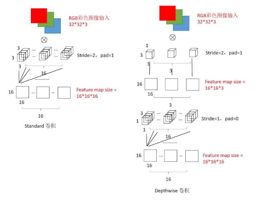
看上面这个图就能知道本文介绍的网络的核心结构在哪里啦？

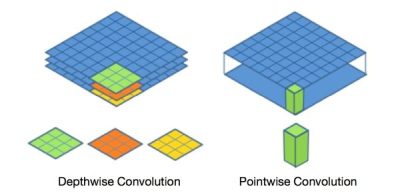
深度可分离卷积提出了一种新的思路：对于不同的输入channel采取不同的卷积核进行卷积，它将普通的卷积操作分解为两个过程。

为了方便大家理解，我们现来看看普通卷积的过程。

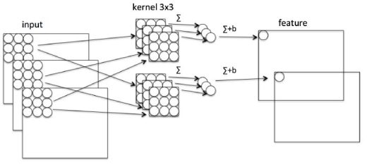
这张图比较清晰，我们按照一个立体的卷积核和原始图像进行卷积，然后获得若干个feather map。

接下来是MobileNet的卷积过程，MobileNet卷积过程一般分为两个步骤

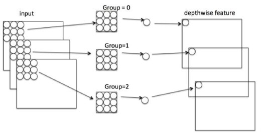
Depthwise

Depthwise是指将 $N\times H\times W \times C$ 的输入分为 $group=C$ 组，然后每一组做 $3 \times 3$ 卷积。这样相当于收集了每个Channel的空间特征，即Depthwise特征。

Pointwise

Pointwise是指对 $N\times H\times W \times C$ 的输入做 $k$ 个普通的 $1\times1$ 卷积。这样相当于收集了每个点的特征，即Pointwise特征。Depthwise+Pointwise最终输出也是 $N \times H\times W \times k$ ,刚好和原始的卷积一次结构保持一致。

分析

经过上面这个过程究竟带来这什么好处呢？

其实最核心的优化就是参数急剧下降，准确率没有明显的下滑，所以也就是MobileNet这个名字的由来，也可以在手机上运行。

举个栗子

需求：假设输入通道数为3，要求输出通道数为256。

对比一下不同卷积的乘法次数：

普通卷积计算量为： $H\times W \times C\times k \times 3\times 3$
Depthwise计算量为： $H\times W \times C \times 3\times 3$
Pointwise计算量为： $H\times W\times C\times k$

通过Depthwise+Pointwise的拆分，相当于将普通卷积的计算量压缩为：

\frac{Depthwise + Pointwise}{conv} =\frac{1}{k} \tag{1.1}

也就是将原有的参数压缩了 $\frac{1}{k}$ ,然后还带来了另外的一个优点，如下。

通道区域分离

深度可分离卷积将以往普通卷积操作同时考虑通道和区域改变（卷积先只考虑区域，然后再考虑通道），实现了通道和区域的分离。

代码实现

import tensorflow as tf

img1 = tf.constant(value=[[[[1], [2], [3], [4]],
                           [[1], [2], [3], [4]],
                           [[1], [2], [3], [4]],
                           [[1], [2], [3], [4]]]], dtype=tf.float32)
img2 = tf.constant(value=[[[[1], [1], [1], [1]],
                           [[1], [1], [1], [1]],
                           [[1], [1], [1], [1]],
                           [[1], [1], [1], [1]]]], dtype=tf.float32)
img = tf.concat(values=[img1, img2], axis=3)
## img's shape is (1, 4, 4, 2)
filter1 = tf.constant(value=0, shape=[3, 3, 1, 1], dtype=tf.float32)
filter2 = tf.constant(value=1, shape=[3, 3, 1, 1], dtype=tf.float32)
filter3 = tf.constant(value=2, shape=[3, 3, 1, 1], dtype=tf.float32)
filter4 = tf.constant(value=3, shape=[3, 3, 1, 1], dtype=tf.float32)
filter_out1 = tf.concat(values=[filter1, filter2], axis=2)
filter_out2 = tf.concat(values=[filter3, filter4], axis=2)
filter = tf.concat(values=[filter_out1, filter_out2], axis=3)
out_img_depthwise = tf.nn.depthwise_conv2d(input=img,
                                           filter=filter, strides=[1, 1, 1, 1],
                                           rate=[1, 1], padding='VALID')
point_filter = tf.constant(value=1, shape=[1, 1, 4, 4], dtype=tf.float32)
out_img_s = tf.nn.conv2d(input=out_img_depthwise, filter=point_filter, strides=[1, 1, 1, 1], padding='VALID')
with tf.Session() as sess:
    res3 = sess.run(out_img_s)

# out_img_s = tf.nn.separable_conv2d(input=img,
#                                     depthwise_filter=filter,
#                                     pointwise_filter=point_filter,
#                                     strides=[1,1,1,1], rate=[1,1], padding='VALID')

以上就是一个简单的mobile net实现的过程，最后几行的注释是合并的上面提到的Depthwise和Pointwise操作合并成一层。